VOLTAGE AND CURRENT RELATIONS INVOLVING SHORT TRANSMISSION LINES

Short Transmission Line

The equivalent circuit and vector diagram of a short transmission line are shown in the figure given below.In the equivalent circuit short transmission line is represented by the lumped parameters R and L. R is the resistance (per phase) L is the inductance (per phase) of the entire transmission line.As said earlier the effect of shunt capacitance and conductance is not considered in the equivalent circuit.The line is shown to have two ends : sending end (designated by the subscript S) at the generator, and the receiving end (designated R) at the load.

The phasor diagram is drawn taking Ir, the receiving end current as the reference.

The terms with in the simple brackets is small as compared to unity, using binomial expansion and limiting only to second term

Vs ≈ Vr + IrR cosΦr + IrX sinΦr

Here Vs is the sending end voltage corresponding to a particular load current and power factor condition. It can be seen from the equivalent circuit that the receiving end voltage under no load is same as the sending end voltage under full load condition i.eVr(no 

 

load) = Vs . Therefore where Vr and Vx are the per unit values of resistance and reactance of the line.From the equivalent circuit diagram we can observe that

Vs = Vr + Ir ( R + jX) = Vr + IrZ

Is = Ir

In a four terminal passive network the voltage and current on the receiving end and sending end are related by following pair of equations

Vs = AVr + BIr

Is = CVr + DIr

Comparing the above two sets of equations, for a short transmission line A = 1, B = Z, C = 0, D = 1. ABCD constants can be used for calculation of regulation of the line as follows:

Normally the quantities P,Ir and cosΦr at the receiving end are given and ofcourse the ABCD constants.Then determine sending end voltage using the relation Vs = AVr + BIr. Vr(no load) at the receivind end is given by Vs/A when Ir = 0.

BUNDLED CONDUCTORS INVOLVING CAPACITANCE

The equivalent circuit of a short transmission line is shown in Fig. 5.4,where

Is- sending-end current
Ir- receiving-end current
Vs- sending-end line-to-neutral voltage
Vr- receiving-end line-to-neutral voltage

The circuit is solved as a simple series ac circuit. Since there are no shunt arms, the current is the same at the sending and receiving ends of the line and


The voltage at the sending end is


where Z is zl, the total series impedance of the line.

The effect of the variation of the power factor of the load on the voltage regulation of a line is most easily understood for the short line and therefore will be considered at this time. Voltage regulation of a transmission line is the rise in voltage at the receiving end, expressed in percent of full-load voltage when full load at a specified power factor is removed while the sending-end voltage is held constant. In the form of an equation


where is the magnitude of receiving-end voltage at no load and is the magnitude of receiving-end voltage at full load with constant. After the load on the short transmission line represented by the circuit of Fig. 5.4, is removed, the voltage at the receiving-end is equal to the voltage at the sending-end. In Fig. 5.4, with the load connected, the receiving-end voltage is designated by and . The sending-end voltage is and The phasor diagrams of Fig. 5.5 are drawn for the same magnitudes of receiving-end voltage and current and show that a larger value of sending-end voltage is required to maintain a given receiving-end voltage when the receiving-end current is lagging the voltage than when the same current and voltage are in phase. A still smaller sending-end voltage is required to to maintain the given receiving-end voltage when the receiving-end current leads the voltage. The voltage drop is the same in the series impedance of of the line in all cases, but because of the different power factors the voltage drop is added to the to the receiving-end voltage at a different angle in each case. The regulation is greatest for lagging power factors. The inductive reactance of a transmission line is larger than the resistance, and the principle of regulation illustrated in Fig. 5.5 is true for any load supplied by a predominantly inductive circuit. The magnitude of the voltage drop for a short line have been exaggerated with respect to in drawing the phasor diagrams in order to illustrate the point more clearly. The relation between the power factor and regulations for longer line is similar to that for short lines but is not visualized so easily.

BUNDLED CONDUCTORS INVOLVING CAPACITANCE

Figure 4.10 shows a bundled-conductor line for which we can write an equation for the voltage from conductor a to conductor b. The conductors of any one bundle in parallel, and we can assume the charge per bundle divides equally between the conductors of the bundle since the separation between bundles is usually more than 15 times the spacing between the conductors of the bundle. Also, since D12 is much greater than d, we can use D12 is place of distances D12-d and D12+d make other similar substitutions of bundle separation distances instead of using the more exact expressions that occur in finding Vab. The difference due to this approximation cannot be detected in the final result for usual spacing even when the calculation is carried to five or six significant figures.

If the charge on phase a is qa, conductors a and a' each have the charge qa/2; similar division of charge is assumed for phase b and c. Then








The letters under each logarithmic term indicate the conductor whose charge is accounted for by that therm. Combining terms gives




The is the same as for a two conductor bundle except that r has replaced Ds. This leads us to the very important conclusion that a modified GMD method applies to calculation of capacitance of bundled-conductor three phase line having two conductors per bundle. The modification is that we are using outside radius in place of the GMR of a single conductor.

It is logical to conclude that the modified GMD method applies to other bundling configurations. If we let D stand for the modified GMR to be used in capacitance calculations to distinguish it from D used in inductance calculations, we have


Then for a two-strand bundle


for a three-strand bundle


and for a four-strand bundle

EFFECTS OF EARTH ON THE CAPACITANCE OF THREE PHASE TRANSMISSION LINES

Earth affects the capacitance of a transmission line because its presence alters the electric field of the line. If we assume that the earth is a perfect conductor in the form of a horizontal plane of infinite extent, we realize that the electric field of charged conductors above the earth is not the same as it would be if the equipotential surface of the earth were not present. The electric field of the charged conductors is forced to conform to the presence of the earth's surface. The assumption of a flat, equipotential surface is, of course, limited by the irregularity of terrain and the type of surface of the earth. The assumption enables us, however, to understand the effect of a conducting earth on capacitance calculations.

Consider a circuit consisting of a single overhead conductor with a return path through the earth. In charging the conductor, charges come from the earth to reside on a conductor, and a potential difference exist between the conductor and earth. The earth has a charge equal in magnitude to that on a conductor but of opposite sign. Electric flux from the charges on the conductor to the charges on the earth is perpendicular to the earth's equipotential surface, since the surface is assumed to be a perfect conductor. Let us imagine a fictitious conductor of the same size and shape as the overhead conductor lying directly below the original conductor at a distance equal to twice the distance of the conductor above the plane of the ground. The fictitious conductor is below the surface of the earth by a distance equal to the distance of the overhead conductor above the earth. If the earth is removed and a charge equal and opposite to that on the overhead conductor is assumed on the overhead conductor is assumed on the fictitious conductor, the plane midway between the original conductor and the fictitious conductor is an equipotential surface and occupies the same position as the equipotential surface of the earth. The electric flux between the overhead conductor and this equipotential surface is the same as that which existed between the conductor and the earth. thus, the purposes of calculation of capacitance, the earth may be replaced by a fictitious charged conductor below the surface of the earth by a distance equal to that of the overhead conductor above the earth. Such a conductor has a charge equal in magnitude and opposite in sign to that of the original conductor and is called the image conductor.

The method of calculating the capacitance by replacing the earth by the image of an overhead conductor can be extended to more than one conductor. If we locate an image conductor for each overhead conductor, the flux between the original conductors and their images is perpendicular to the plane which replaces the earth, and that plane is equipotential surface. The flux above the plane is the same as it is when the earth is present instead of the image conductors.



If the conductors is high above ground compared with distances between them, the diagonal distances in the numerator of the correction term are nearly equal to the vertical distances in the denominator and the term is very small. This is the usual case, and the effect of ground is generally neglected for three phase lines except for calculations by symmetrical components when the sum of the three line current is not zero.

CAPACITANCE OF THREE PHASE TRANSMISSION LINES

Capacitance of a transmission line is the result of the potential difference between the conductors; it causes them to be charged in the same manner as the plates of a capacitor when there is a potential difference between them. The capacitance between the conductor is the charge per unit of potential difference. capacitance between parallel conductors is a constant depending on the size and spacing of the conductors. For power lines less than about 80 km (50mi) long the effect of capacitance is slight and is usually neglected. For longer lines of higher voltage, capacitance becomes increasingly important.

An alternating voltage impressed on a transmission line causes the charge on the conductors at any point to increase and decrease with the increase and decrease of the instantaneous value of the voltage between conductors at the point. The flow of charge is current, and the current caused by the alternate charging and discharging of a line due to an alternating voltage is called the charging current of the line. Charging current flows in a transmission line even when it is a open-circuited. It affects the voltage drop along the line as well as the efficiency and power factor of the line and the stability of the system of which the line is a part.

INDUCTANCE OF THREE PHASE TRANSMISSION LINES

Inductance is the property in an electric circuit where a change in the electric current through that circuit induces an electromotive force(Emf) that opposes the change in current

In electrical circuits, any electric current, i, produces a magnetic field and hence generates a total magnetic flux Φ, acting on the circuit. This magnetic flux, due to Lenz's law tends to act to oppose changes in the flux by generating a voltage (a back EMF) in the circuit that counters or tends to reduce the rate of change in the current. The ratio of the magnetic flux to the current is called the self-inductance, which is usually simply referred to as the inductance of the circuit. To add inductance to a circuit, electronic component called inductors are used, which consist of coils of wire to concentrate the magnetic field.

The term 'inductance' was coined by Oliver Heaviside in February 1886. It is customary to use the symbol L for inductance, possibly in honour of the physicist Heinrich Lenz

The unit of inductance is the henry (H), named after American scientist and magnetic researcher Joseph Henry 1 H = 1Wb/A.

Definitions

The quantitative definition of the (self-) inductance of a wire loop in SI units ( webers per ampere known as henries is

where L is the inductance, Φ denotes the magnetic flux through the area spanned by the loop, Ni is the current in amperes. The flux linkage thus is is the number of wire turns, and

Properties of inductance

Taking the time derivative of both sides of the equation NΦ = Li yields:

In most physical cases, the inductance is constant with time and so

By Faraday's law of Induction we have:

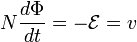
where is the Electromotive force (emf) and v is the induced voltage. Note that the emf is opposite to the induced voltage. Thus:

or

Bundled conductors

At extra-high (EHV), that is, voltages above 230 kV, corona with its resultant power loss and particularly its interference with communications is excessive if the circuit has only one conductor per phase. The high-voltage gradient at the conductor in the EHV range is reduced considerably by having two or more conductors per phase in close proximity copared with the spacing between phases. Such a line is said to be composed of bundled conductors. The bundle consists of two, three or four conductors. The three conductor bundle usually has the conductors at the vertices of an equilateral triangle, and the four conductor bundle usually has its conductors at the corners of a square. The current will not devide exactly between the conductors of the bundle unless there is a transposition of the conductors within the bundles, but the difference is of no practical imporatnce, and the GMD method is accurate for caculations.

Reduced reactance is the equally important advantage of bundling. Increacing the number of conductors in the bundle reduces the effects of corona and reduces the reactance. The reduction of reactance results from the increased GMR of the bundle. The calculation of GMR is, of course, exactly the same as that of a stranded conductor. Each conductor of a two-conductor bundle, for instance, is treated as one strand of a two-strand conductor. If we let indicate the GMR of a bundle conductor and the GMR of the individual conductors composing the bundle.

For a two-strand bundle

==

For a three-strand bundle

=

For a four-strand bundle

POWER TRANSMISSION AND DISTRIBUTION

The voltage of large generators usually is in the range of 13.8 kV to 24kV. Large modern generators, however, are built for voltages ranging from 18-24kV. No standard for generator voltages has been adopted.

Diagram of an electrical system.

Electric power transmission or "high voltage electric transmission" is the bulk transfer of electrical energy, from generating plants (historically hydroelectric, nuclear or coal fired but now also wind, solar, geothermal and other forms of renewable energy) to substations located near to population centers. This is distinct from the local wiring between high voltage substations and customers, which is typically referred to as electricity distribution.

Transmission lines, when interconnected with each other, become high voltage transmission networks. In the US, these are typically referred to as "power grids" or sometimes simply as "the grid". North America has three major grids: The Western Interconnect; The Eastern Interconnect and the Electric Reliability Council of Texas (or ERCOT) grid.

Historically, transmission and distribution lines were owned by the same company, but over the last decade or so many countries have introduced market reforms that have led to the separation of the electricity transmission business from the distribution business.

Transmission lines mostly use three phase alternating current (AC), although single phase AC is sometimes used in railway electrification systems. High-voltage direct current (HVDC) technology is used only for very long distances (typically greater than 400 miles); undersea cables (typically longer than 30 miles); or for connecting two AC networks that are not synchronized.

Electricity is transmitted at high voltages (110 kV or above) to reduce the energy lost in long distance transmission. Power is usually transmitted through overhead power lines. Underground power transmission has a significantly higher cost and greater operational limitations but is sometimes used in urban areas or sensitive locations.

A key limitation in the distribution of electricity is the difficulty in storing significant quantities of electrical energy. A sophisticated system of control is therefore required, to ensure electric generation very closely matches the demand. If supply and demand are not in balance, generation plants and transmission equipment can shut down which, in the worst cases, can lead to a major regional blackout, such as occurred in Cal ifornia and the US Northwest in 1996 and in the US Northeast in 1965, 1977 and 2003. To reduce the risk of such failures, electric transmission networks are interconnected into regional, national or continental wide networks thereby providing multiple redundant alternate routes for power to flow should (weather or equipment) failures occur. Much analysis is done by transmission companies to determine the maximum reliable capacity of each line which is mostly less than its physical or thermal limit, to ensure spare capacity is available should there by any such failure in another part of the network.

Transmission lines

TRANSMISSION SYSTEM

It includes all land conversion, structures and equipment at a primary source of supply,
line switching and conversion stations between generating or receiving point and the
entrance to a distribution center or wholesale point. All lines equipment whose primary
purpose is to augment, integrate or tie together sources of power supply.

DISTRIBUTION SYSTEM

It connects all individual loads to the transmission line at a substation which performs
voltage transmission and switching function.

Purpose of transmission

1. To transmit power from water power site to a market. These may be very long justified because of subsidy aspect connected with a project. 2. For bulk power to a load center from outlying steam station these are likely to be relatively short. 3. For interconnection purposes, transfer of energy from one system to another in case of emergency or in response to diversity in system peaks.

COURSE SYLLABUS

I. Department: ELECTRICAL AND ALLIED DEPARTMENT

II. Course Code: EE 11

III. Course Title: Power System

IV. Course Description:
The course discusses electrical power generation, transmission, and distribution systems for electrical engineering students. It also discusses the principles of AC/DC transmission and distribution system. It deals also with the study of the calculation of parameters, conductor selection and underground power transmission and distribution.


V. Course Objectives:


At the end of the course, the student shall be able to:

a. Understand a broad range of topics in the power systems.
b. Learn the basic theories and applications in the power systems.
c. Promote their interest in learning more about the electric power industry with emphasis on electric power transmission lines.
d. Solve problems involving short, medium and long transmission lines.
e. Impart the basic foundations of electric power system from which he/she can continue his education while at work in the field.

VI. Unit Credit/Time: 3 units lecture(3.75hours/week; 14 weeks/term)

VII. Semester/Term Offered: 3rd year/second term

VIII. Pre-requisite Subjects:EE3/EE3L

IX. Co-requisite Subject: EE 11L

X. Clientele: BSEE Straight Engineering Students

XI. Requirements:
The requirements of this course and the corresponding inputs into the final grade are as follows:

a. Quizzes, seat works, assignments, recitation, attendance ... 20%
b. Unit Test and actual exercises ............................................... 25%
c. Term Test .................................................................................. 20%
d. Laboratory ................................................................................ 35%
Total ............................................................................................ 100%

XII. Grading System:
Ratings in the quizzes/exercises, homeworks, seat works, unit test, term test and other requirements may be in the 0-100% or the 0-10 scale, wherein 10 is the highest, 0 is the lowest and 5 is the minimum passing.

Whatever scale used, all final grades are transmuted to the 1-5 scale using the following conversion, with 1.00 as EXCELLENT and 5.00 as FAILED.


XIII. Textbook/s:

Stevenson, William Jr. D. Elements of Power System Analysis. 4th Edition New York; Mc Graw Hill Book Company, C 1984

TRANSMISSION LINE PARAMETERS

An electric transmission line has four parameters which affect its ability to fulfill its function as part of a power system: resistance, inductance, capacitance, and conductance.

Conductance between conductors or between conductors and the ground accounts for the leakage current at the insulators of overhead lines and through the insulation of cables. Since leakage at insulators of overhead lines is negligible, the conductance between conductors of an overhead line is assumed to be zero.

Capacitance exists between the conductors and is the charge on the conductors per unit of potential difference between them.

The resistance and inductance uniformly distributed along the line form the series impedance. The conductance and capacitance existing between conductors of a single-phase line or from a conductor to neutral of a three-phase line form the shunt admittance.

TYPES OF CONDUCTORS

Symbols identifying different types of aluminum conductors are as follows:

AAC- all-aluminum conductors
AAAC- all-aluminum alloy conductors
ACSR- aluminum conductor, steel reinforced
ACAR- aluminum conductor, alloy reinforced

Aluminum alloy conductors have higher tensile strength than the ordinary electrical-conductor grade of aluminum. ACSR consists of a central core of steel strands surrounded by layers of aluminum strands. ACAR has a central core of higher-strength aluminum surrounded by layers of electrical-conductor-grade aluminum.

RESISTANCE ON TRANSMISSION LINES

DC resistance

The resistance R of a conductor of uniform cross section can be computed as

where:

l is the length of the conductor, measured in meters [m]

A is the cross-sectional area of the current flow, measured in square meters [m²]

ρ (Greek: rho) is the electrical resistivity (also called specific electrical resistance) of the material, measured in Ohm · meter (Ω m). Resistivity is a measure of the material's ability to oppose electric current.

For practical reasons, any connections to a real conductor will almost certainly mean the current density is not totally uniform. However, this formula still provides a good approximation for long thin conductors such as wires.

Temperature dependence

Near room temperature, the electric resistance of a typical metal increases linearly with rising temperature, while the electrical resistance of a typical semiconductor decreases with rising temperature. The amount of that change in resistance can be calculated using the temperature coefficient of resistivity of the material using the following formula:

where:

T is its temperature,

T₀ is a reference temperature (usually room temperature),

R₀ is the resistance at T₀, and

α is the percentage change in resistivity per unit temperature.

The constant α depends only on the material being considered. The relationship stated is actually only an approximate one, the true physics being somewhat non-linear, or looking at it another way, α itself varies with temperature. For this reason it is usual to specify the temperature that α was measured at with a suffix, such as α₁₅ and the relationship only holds in a range of temperatures around the reference.

This table shows the resistivity and temperature coefficient of various materials at 20 °C (68 °F)

Material------- Resistivity (Ω·m) at 20 °C----- Temperature coefficient* [K−1]
Silver------------ 1.59×10−8-------------------------------- 0.0038
Copper--------- 1.72×10−8-------------------------------- 0.0039
Gold------------- 2.44×10−8-------------------------------- 0.0034
Aluminium----- 2.82×10−8-------------------------------- 0.0039
Calcium-------- 3.36x10−8
Tungsten------- 5.60×10−8------------------------------- 0.0045
Zinc-------------- 5.90×10−8------------------------------- 0.0037
Nickel----------- 6.99×10−8
Iron-------------- 1.0×10−7---------------------------------- 0.005
Platinum------- 1.06×10−7-------------------------------- 0.00392
Tin--------------- 1.09×10−7-------------------------------- 0.0045
Lead------------ 2.2×10−7---------------------------------- 0.0039
Manganin----- 4.82×10−7-------------------------------- 0.000002
Constantan---- 4.9×10−7--------------------------------- 0.000 008
Mercury-------- 9.8×10−7---------------------------------- 0.0009
Nichrome[6]-- 1.10×10−6--------------------------------- 0.0004
Carbon[7]----- 3.5×10−5--------------------------------- −0.0005
Germanium[7]-- 4.6×10−1------------------------------- −0.048
Silicon[7]------ 6.40×10-2-------------------------------- −0.075

VOLTAGE AND CURRENT RELATIONS INVOLVING MEDIUM TRANSMISSION LINES

VOLTAGE AND CURRENT RELATIONS INVOLVING LONG TRANSMISSION LINES

MECHANICAL CONSIDERATION ON TRANSMISSION LINES